ragavi-vis

This is the visibility plotter. Supported arguments are as follows

xaxis	yaxis	iter-axis	colour-axis
amplitude	amplitude	antenna	antenna1
antenna1	phase	antenna1	antenna2
antenna2	real	antenna2	spw
channel	imaginary	baseline	baseline
frequency		corr	corr
imaginary		field	field
phase		scan	scan
real		spw
scan
time
uvdistance (uv distamce m)
uvwave (uv distance lambda)

Some of the arguments can be shortened using the following aliases

axis	alias
amplitude	amp
antenna	ant
antenna1	ant1
antenna2	ant2
baseline	bl
channel	chan
frequency	freq
imaginary	imag
uvdistance	uvdist
uvwave	uvidistl / uvdist_l

Iteration can also be activated through the -ia / --iter-axis option. It is also possible to colour over some axis (most of the iteration axes are supported as shown in the table above) and this can be activated through the -ca / --colour-axis argument. Please note that the mandatory arguments are --xaxis, --yaxis, --ms.

Note

Output files genrated by ragavi-vis can be very large for iterated plots because of the resolution of each generated plot. For this reason, unless --canvas-width and --canvas-height are explicitly provided, ragavi-gains will automatically shrink the canvas sizes to 200 by 200 in order to minimise the resulting output.

Averaging

ragavi-vis has the ability to perform averaging before a plot is generated, by specifying the --cbin or --tbin arguments. These enable channel averaging and time averaging respectively. It is made possible through the use of the Codex africanus averaging API.

Averaging is performed over per SPW, FIELD and Scan. This means that data is grouped by DATA_DESC_ID, FIELD_ID and SCAN_NUMBER beforehand. However, data selection (such as selection of spws, fields, scans and baselines to be present) is done before the averaging to avoid processing data that is unnecessary for the plot.

Computing Resources

Number of computer cores to be used, memory per core and the size of chunks to be loaded to each core may also be specified using -nc / --num-cores, -ml / --memory-limit and -cs / --chunk-size respectively. These may play an active role in improving the performance and memory management as ragavi-vis runs. However, finding an optimal combination may be a tricky task but is well worth while.

By default, ragavi-vis will use a maximum of 10 cores, with the maximum memory associated to each core being 1GB, and a chunk size in the row axis as 5000. The number of cores to be used, however, is dependent on the amount of RAM that is available on the host machine, in order to try and ensure that:

Number of cores x memory limit per core < total amount of available RAM

This means that, if the number of cores is less than 10, then by default, ragavi-vis will attempt to match the number of cores to those available. Given that visibility data has the shape (rows x channels x correlations), chunk sizes may also be chosen per each dimension using comma separated values (see the help section on this page). As mentioned, the default chunk size is 5000 in the row axis, while the chunks sizes in the rest of the dimension are determined by the sizes of those dimensions (hence remaining as they are). Therefore, the true size of the chunks during processing will be translated to (nrows x nchannels x ncorrelations).

It is worth noting that supplying the x-axis and y-axis minimums and maximums may also significantly cut down the plotting time. This is because for minimum and maximum values to be calculated, ragavi-vis’ backends must pass through the entire dataset at least once before plotting begins and again as plotting continues, therefore, taking a longer time. While the effect of this may be minimal in small datasets, it is certainly amplified in large datasets.

Help

The output of the help is as follows:

  usage: ragavi-vis [options] <value>

  optional arguments:
    -h, --help            show this help message and exit
    -v, --version         show program's version number and exit

  Required arguments:
    --ms  [ ...]          MS to plot. Default is None
    -x , --xaxis          X-axis to plot
    -y , --yaxis          Y-axis to plot

Plot settings:
  -ch , --canvas-height
                        Set height resulting image. Note: This is not the plot
                        height. Default is 720
  -cw , --canvas-width
                        Set width of the resulting image. Note: This is not
                        the plot width. Default is 1080.
  --cmap                Colour or colour map to use.A list of valid cmap
                        arguments can be found at:
                        https://colorcet.pyviz.org/user_guide/index.html Note
                        that if the argument "colour-axis" is supplied, a
                        categorical colour scheme will be adopted. Default is
                        blue.
  --cols                Number of columns in grid if iteration is active.
                        Default is 9.
  -ca , --colour-axis   Select column to colourise by. This will result in a
                        single image. Default is None.
  --debug               Enable debug messages
  -ia , --iter-axis     Select column to iterate over. This will result in a
                        grid. Default is None.
  -lf , --logfile       The name of resulting log file (with preferred
                        extension) If no file extension is provided, a '.log'
                        extension is appended. The default log file name is
                        ragavi.log
  -o , --htmlname       Output HTML file name (without '.html')

Data Selection:
  -a , --ant            Select baselines where ANTENNA1 corresponds to the
                        supplied antenna(s). "Can be specified as e.g. "4",
                        "5,6,7", "5~7" (inclusive range), "5:8" (exclusive
                        range), 5:(from 5 to last). Default is all.
  --chan                Channels to select. Can be specified using syntax i.e
                        "0:5" (exclusive range) or "20" for channel 20 or
                        "10~20" (inclusive range) (same as 10:21) "::10" for
                        every 10th channel or "0,1,3" etc. Default is all.
  -c , --corr           Correlation index or subset to plot. Can be specified
                        using normal python slicing syntax i.e "0:5" for
                        0<=corr<5 or "::2" for every 2nd corr or "0" for corr
                        0 or "0,1,3". Can also be specified using comma
                        separated corr labels e.g 'xx,yy' or specifying 'diag'
                        / 'diagonal' for diagonal correlations and 'off-diag'
                        / 'off-diagonal' for of diagonal correlations. Default
                        is all.
  -dc , --data-column   MS column to use for data. Default is DATA.
  --ddid                DATA_DESC_ID(s) /spw to select. Can be specified as
                        e.g. "5", "5,6,7", "5~7" (inclusive range), "5:8"
                        (exclusive range), 5:(from 5 to last). Default is all.
  -f , --field          Field ID(s) / NAME(s) to plot. Can be specified as
                        "0", "0,2,4", "0~3" (inclusive range), "0:3"
                        (exclusive range), "3:" (from 3 to last) or using a
                        field name or comma separated field names. Default is
                        all
  -if, --include-flagged   Include flagged data in the plot. (Plots both flagged
                        and unflagged data.)
  -s , --scan           Scan Number to select. Default is all.
  --taql                TAQL where
  --xmin                Minimum x value to plot
  --xmax                Maximum x value to plot
  --ymin                Minimum y value to plot
  --ymax                Maximum y value to plot

Averaging settings:
  --cbin                Size of channel bins over which to average .e.g
                        setting this to 50 will average over every 5 channels
  --tbin                Time in seconds over which to average .e.g setting
                        this to 120.0 will average over every 120.0 seconds

Resource configurations:
  -cs , --chunks        Chunk sizes to be applied to the dataset. Can be an
                        integer e.g "1000", or a comma separated string e.g
                        "1000,100,2" for multiple dimensions. The available
                        dimensions are (row, chan, corr) respectively. If an
                        integer, the specified chunk size will be applied to
                        all dimensions. If comma separated string, these chunk
                        sizes will be applied to each dimension respectively.
                        Default is 5,000 in the row axis.
  -ml , --mem-limit     Memory limit per core e.g '1GB' or '128MB'. Default is
                        1GB
  -nc , --num-cores     Number of CPU cores to be used by Dask. Default is 10
                        cores. Unless specified, however, this value may
                        change depending on the amount of RAM on this machine
                        to ensure that: num-cores * mem-limit < total RAM
                        available

Examples

Some example plots generated by ragavi-vis

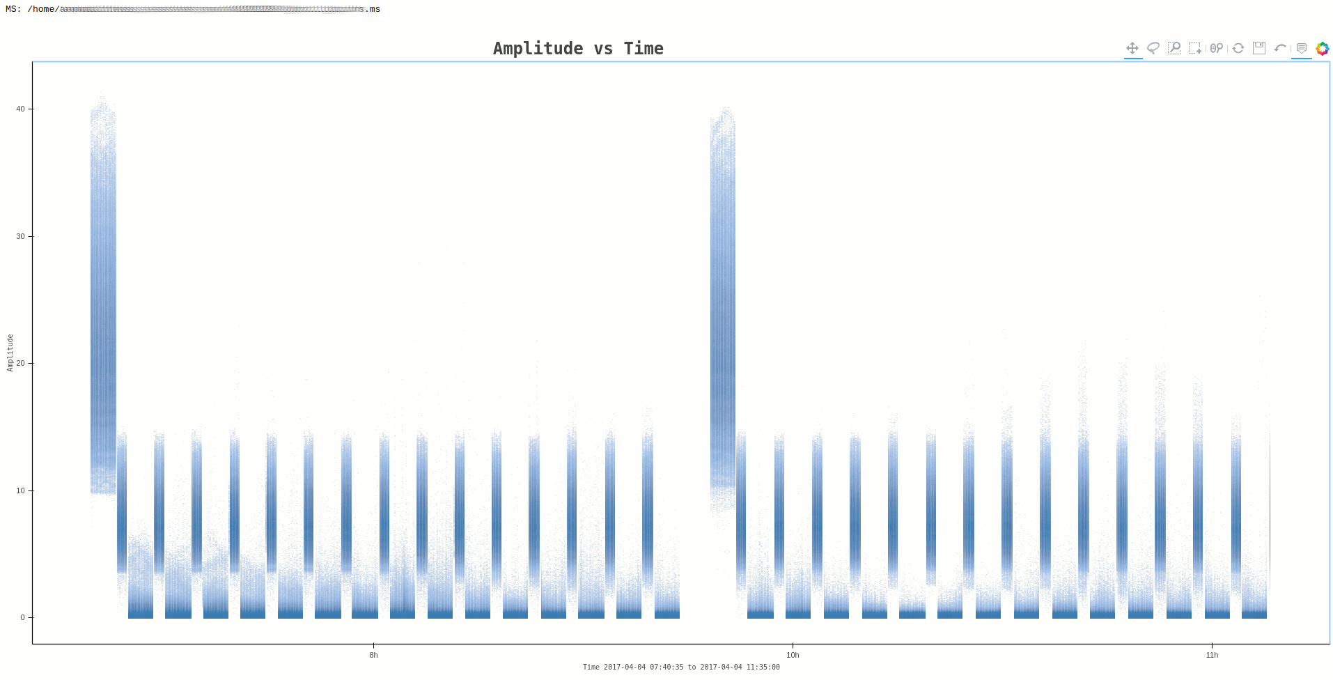
Command: ragavi-vis --ms dir/test.ms --xaxis time --yaxis amp

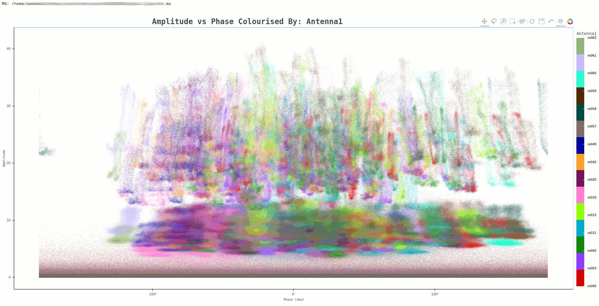
Command: ragavi-vis --ms dir/test.ms --xaxis phase --yaxis amp --colour-axis antenna1

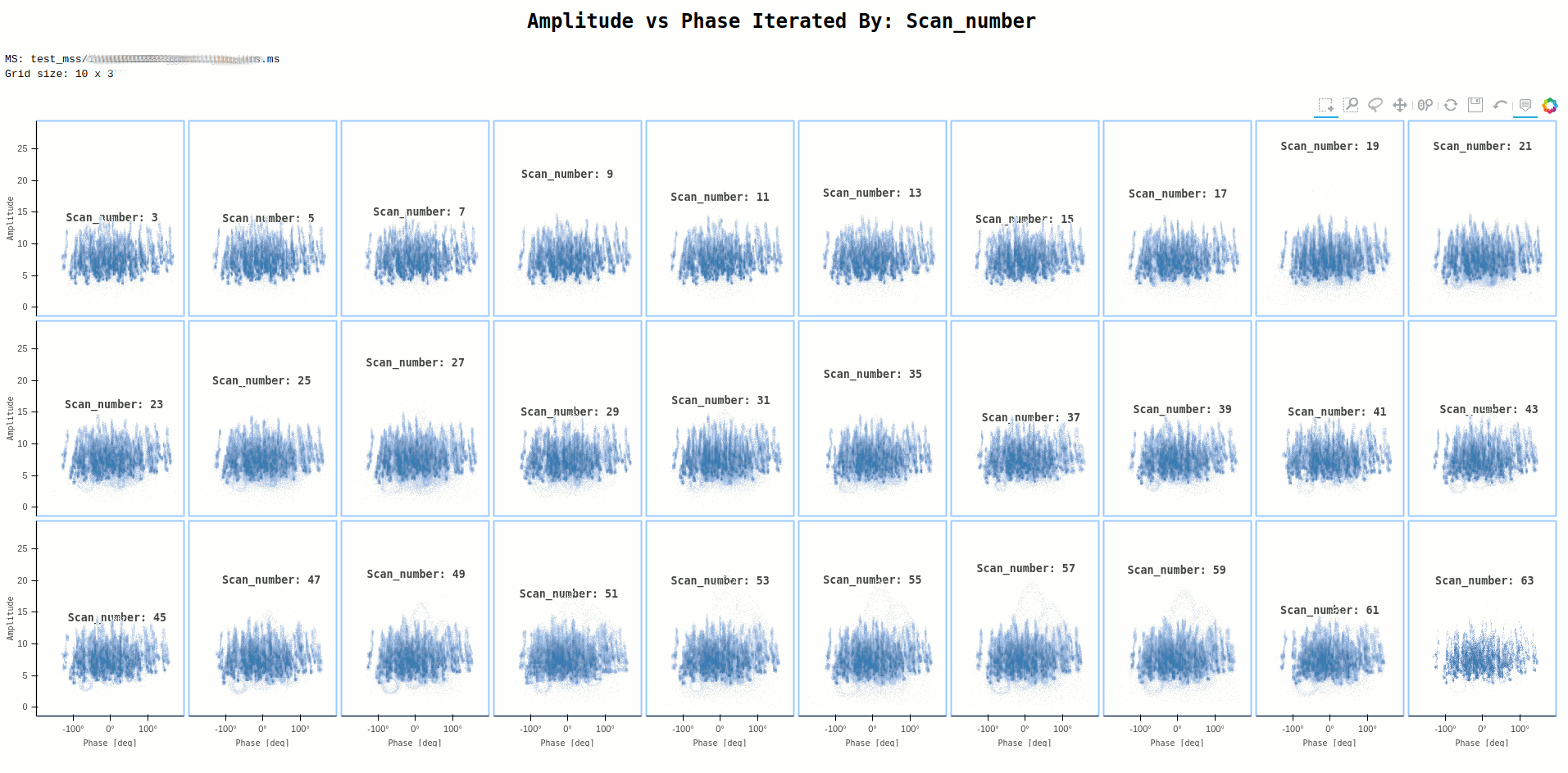
Command: ragavi-vis --ms dir/test.ms --xaxis phase --yaxis amp --iter-axis scan

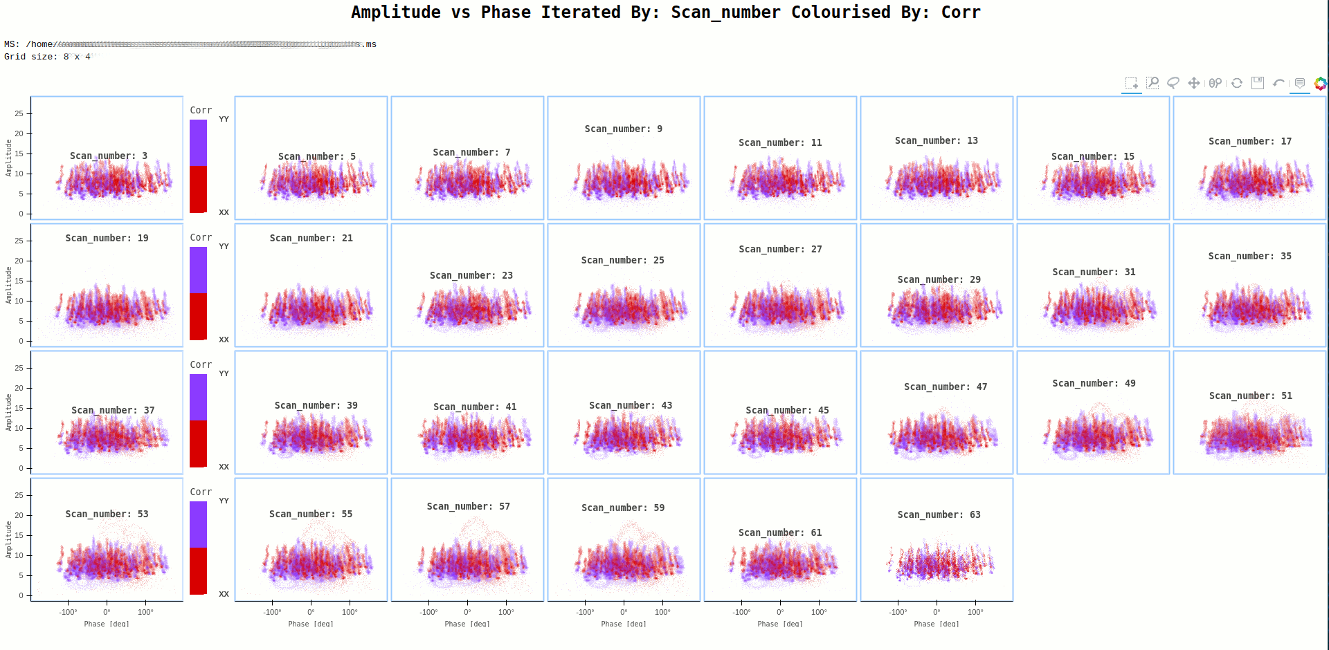
Command: ragavi-vis --ms dir/test.ms --xaxis phase --yaxis amp --iter-axis scan --colour-axis corr

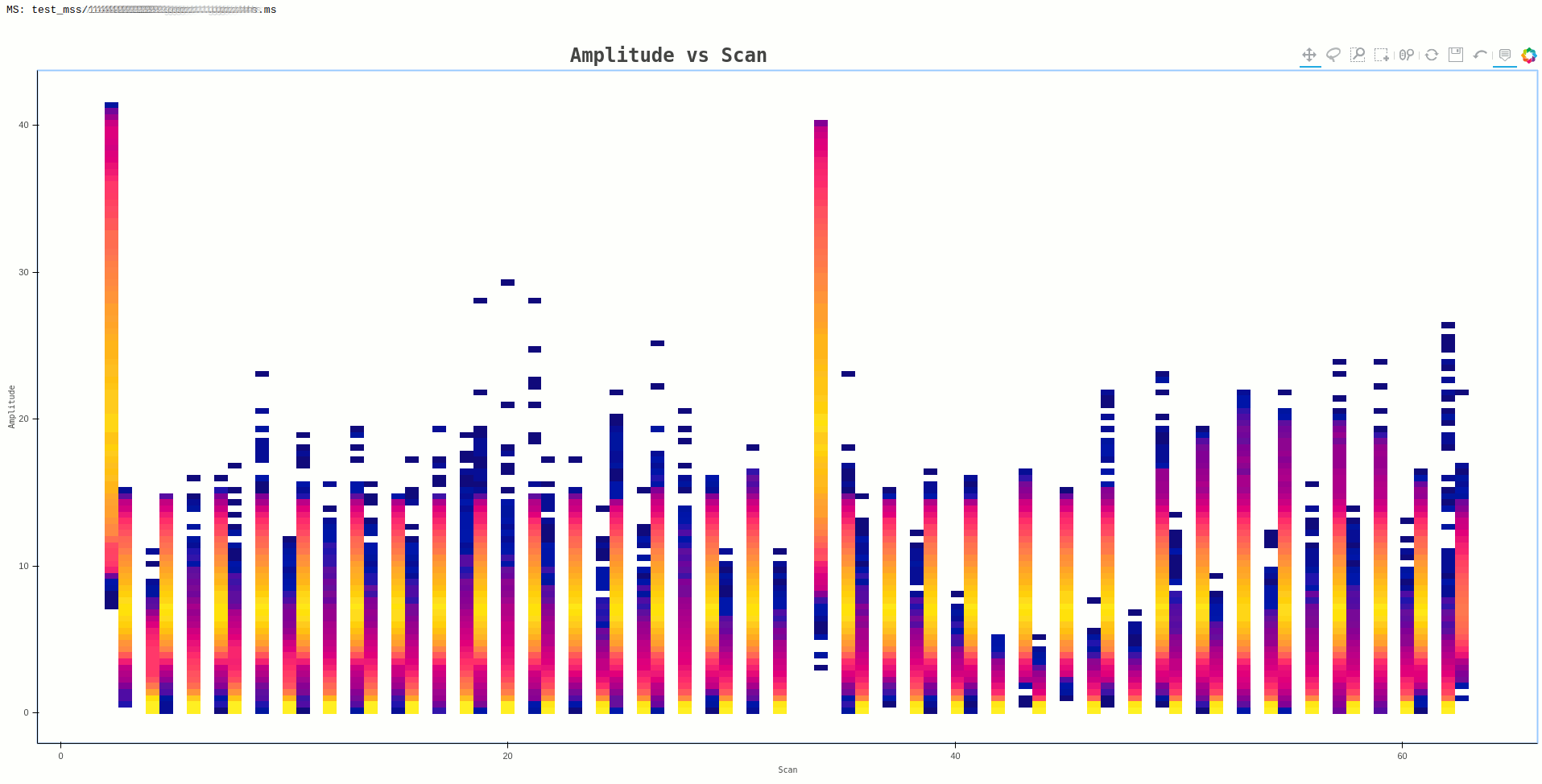
In some cases, the plot generated may have data points that are small and bordering invisible, such as the one below

Command: ragavi-vis --ms dir/test.ms --xaxis scan --yaxis amp --cmap bmy

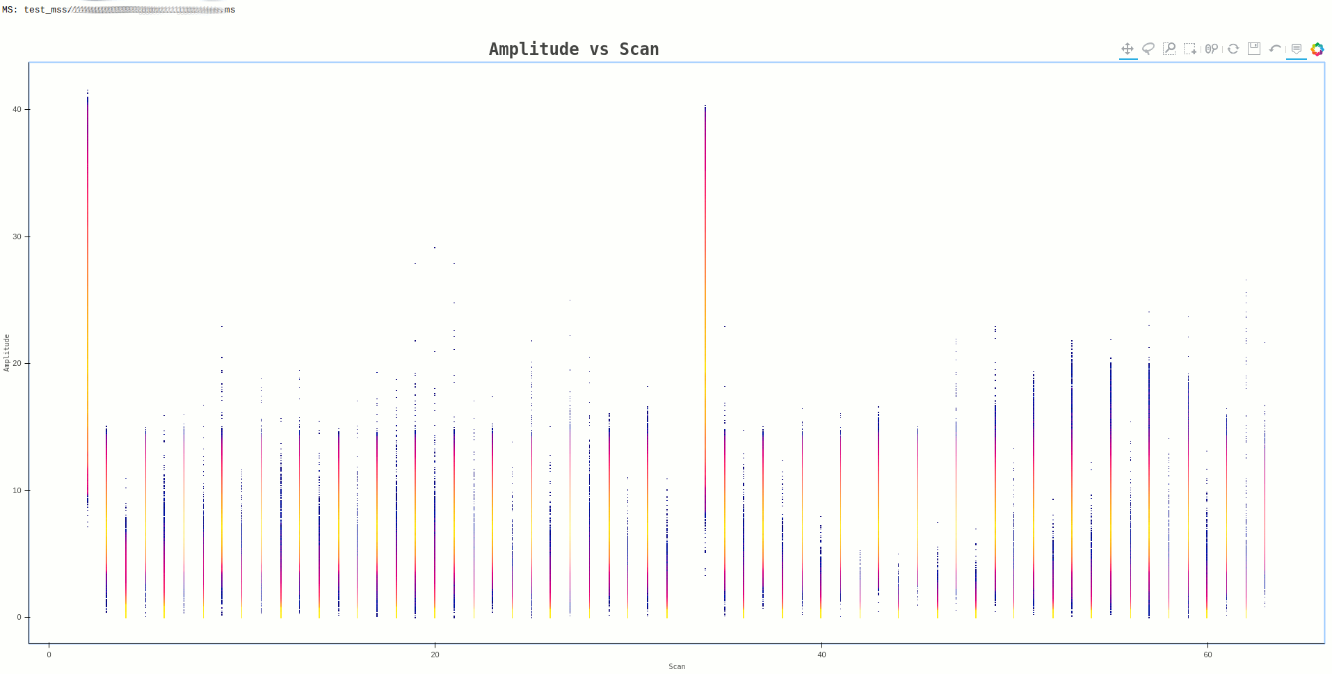
A work around for such a case, is to reduce the resolution of the resulting image, by providing the --canvas-width and --canvas-height arguments. The image above, was generating using the default values 1080 and 720 respectively. If this is changed to 100 and 100, the resulting plot albeit coarse, is clearer as shown below

Command: ragavi-vis --ms dir/test.ms --xaxis scan --yaxis amp --cmap bmy --canvas-width 100 --canvas-height 100