`ragavi-gains`¶

To be used for gain table visualisation.

Currently, gain tables supported for visualisation by ragavi-gains are :

Flux calibration (F tables)

Bandpass calibration (B tables)

Delay calibration (K tables)

Gain calibration (G tables)

D-Jones Leakage tables (D tables)

Pol-cal tables (Kcross, Xf, Df)

Mandatory argument is --table.

If a field name is not specified to ragavi-vis all the fields will be plotted by default. This is the same for correlations and spectral windows.

It is possible to place multiple gain table plots of different [or same] types into a single HTML document using ragavi This can be done by specifying the table names as a space separate list as below

$ragavi-gains --table table/one/name table/two/name table/three/name table/four/name --fields 0

This will yield an output HTML file, with plots in the order

–table	field	gain
table1	0	B
table2	0	G
table3	0	D
table4	0	F

Note

At least a single field, spectral window and correlation must be selected in order for plots to show up.
While antenna data can be made visible through clicking its corresponding legend, this behaviour is not linked to the field, SPW, correlation selection checkboxes. Therefore, clicking the legend for a specific antenna will make data from all fields, SPWs and correlation for that antenna visible. As a workaround, data points can be identified using tooltip information
Unless all the available fields, SPWs and correlations have not been selected, the antenna legends will appear greyed-out. This is because a single legend is attached to multiple data for each of the available categories. Therefore, clicking on legends without meeting the preceeding condition may lead to some awkward results (a toggling effect).

By default, ragavi-gains automatically determines an appropriate x-axis for a given input table. This behaviour can be changed by specifying the -x/xaxis argument.

Use in Jupyter Notebooks¶

To use ragavi-gains in a notebook environment, run in a notebook cell

from ragavi.ragavi import plot_table

#specifying function arguments
args = dict(mytabs=[], cmap='viridis', doplot='ri', corr=1, ant='1,2,3,9,10')

#inline plotting will be done
plot_table(**args)

Generating Static (Non-Interactive) Images¶

It is possible to generate png, ps, pdf, svg with ragavi-gains via two methods. The first method involves generating the HTML format first and then using the save tool found in the toolbar to download the plots. This method requires minimal effort although it may be a necessary redundancy to achieve the static image goal.

The second method involves supplying the --plotname argument, including the desired file extension. For example, --plotname test.png. If only this argument is supplied, then only a single static plot is generated. In case of multiple tables, multiple static files will be generated. However, in case one wants both static and interactive plots, both --htmlname and

--plotname must be supplied.

By default, ragavi uses the canvas image backend for interactive plots, due to performance issues associated with SVG image backend as stated in the Bokeh docs. The default plots generated are always in HTML format.

Warning

If the gain tables supplied contain more than 30,000 points, interactive plots become extremely large and barely interactive (and unresponsive).

In an attempt to overcome this, ragavi-gains generates static plots, in addition to interactive plots, in this case. It is advisable to avoid opening the large (upto hundreds of MBs) HTML as they may cause the browser to hang. Instead, inspect the static plot first and then make an interactive plot containing the antenna / field / corr etc. of your interest by using the selection arguments provided.

Help¶

The full help output for ragavi-gains is:

  usage: ragavi-gains [options] <value>

  A Radio Astronomy Gains and Visibility Inspector

  optional arguments:
    -h, --help            show this help message and exit
    -v, --version         show program's version number and exit

  Required arguments:
    -t   [  ...], --table   [  ...]
                          Table(s) to plot. Multiple tables can be specified as a space separated list

Data Selection:
  -a , --ant            Plot only a specific antenna, or comma-separated list
                        of antennas. Defaults to all.
  -c , --corr           Correlation index to plot. Can be a single integer or
                        comma separated integers e.g '0,2'. Defaults to all.
  --ddid                SPECTRAL_WINDOW_ID or ddid number. Defaults to all
  -f  [ ...], --field  [ ...]
                        Field ID(s) / NAME(s) to plot. Can be specified as
                        "0", "0,2,4", "0~3" (inclusive range), "0:3"
                        (exclusive range), "3:" (from 3 to last) or using a
                        field name or comma separated field names. Defaults to
                        all
  --t0                  Minimum time to plot [in seconds]. Defaults to full
                        range]
  --t1                  Maximum time to plot [in seconds]. Defaults to full
                        range
  --taql                TAQL where clause

Plot settings:
  --cmap                Bokeh or Colorcet colour map to use for antennas. List
                        of available colour maps can be found at: https://docs
                        .bokeh.org/en/latest/docs/reference/palettes.html or
                        https://colorcet.holoviz.org/user_guide/index.html .
                        Defaults to coolwarm
  -d , --doplot         Plot complex values as amplitude & phase (ap) or real
                        and imaginary (ri) or both (all). Defaults to ap.
  --debug               Enable debug messages
  -g [  [  ...]], --gaintype [  [  ...]]
                        Type of table(s) to be plotted. Can be specified as a
                        single character e.g. "B" if a single table has been
                        provided or space separated list e.g B D G if multiple
                        tables have been specified. Valid choices are B D G K
                        & F
  -kx , --k-xaxis       Choose the x-xaxis for the K table. Valid choices are:
                        time or antenna. Defaults to time.
  -lf , --logfile       The name of resulting log file (with preferred
                        extension) If no file extension is provided, a '.log'
                        extension is appended. The default log file name is
                        ragavi.log
  -o , --htmlname       Name of the resulting HTML file. The '.html' prefix
                        will be appended automatically.
  -p , --plotname       Static image name. The suffix of this name determines
                        the type of plot. If foo.png, the output will be PNG,
                        else if foo.svg, the output will be of the SVG format.

Examples¶

This subsection demonstrates the kind of plots that are generated

Interactive plots¶

Command: ragavi-gains --table test.B0 --doplot ap --htmlname test

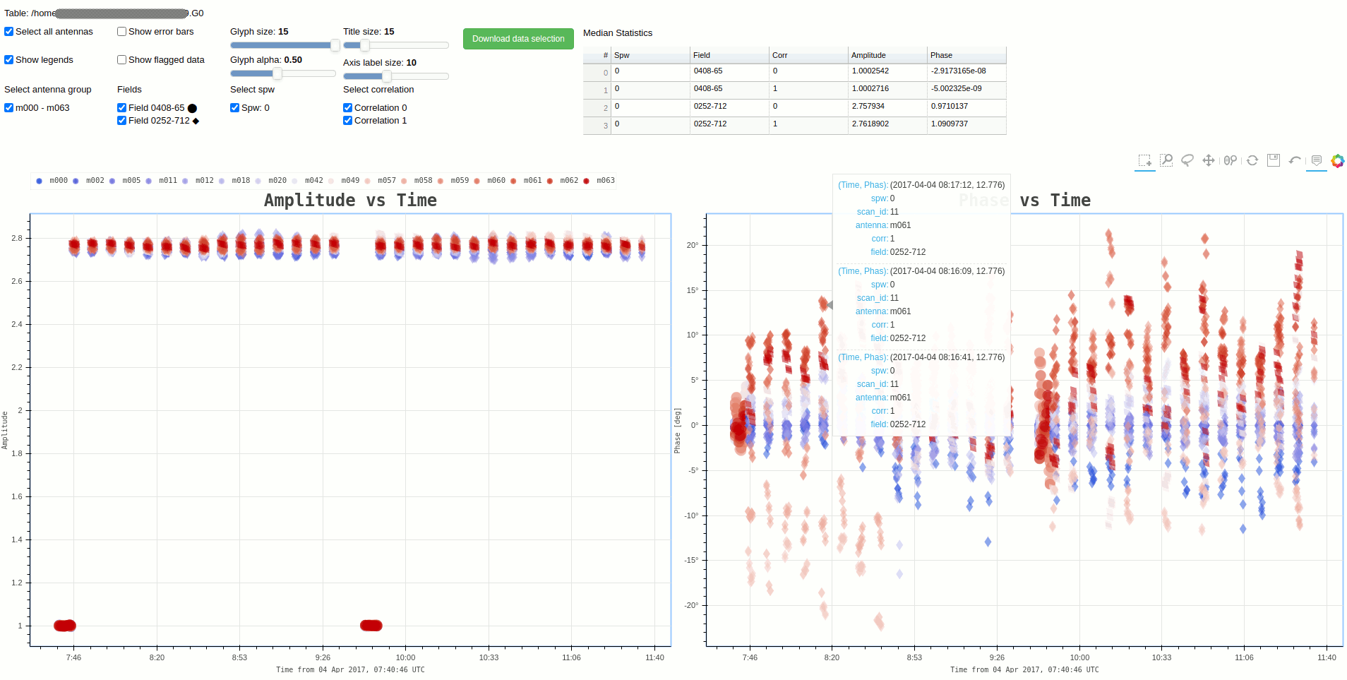
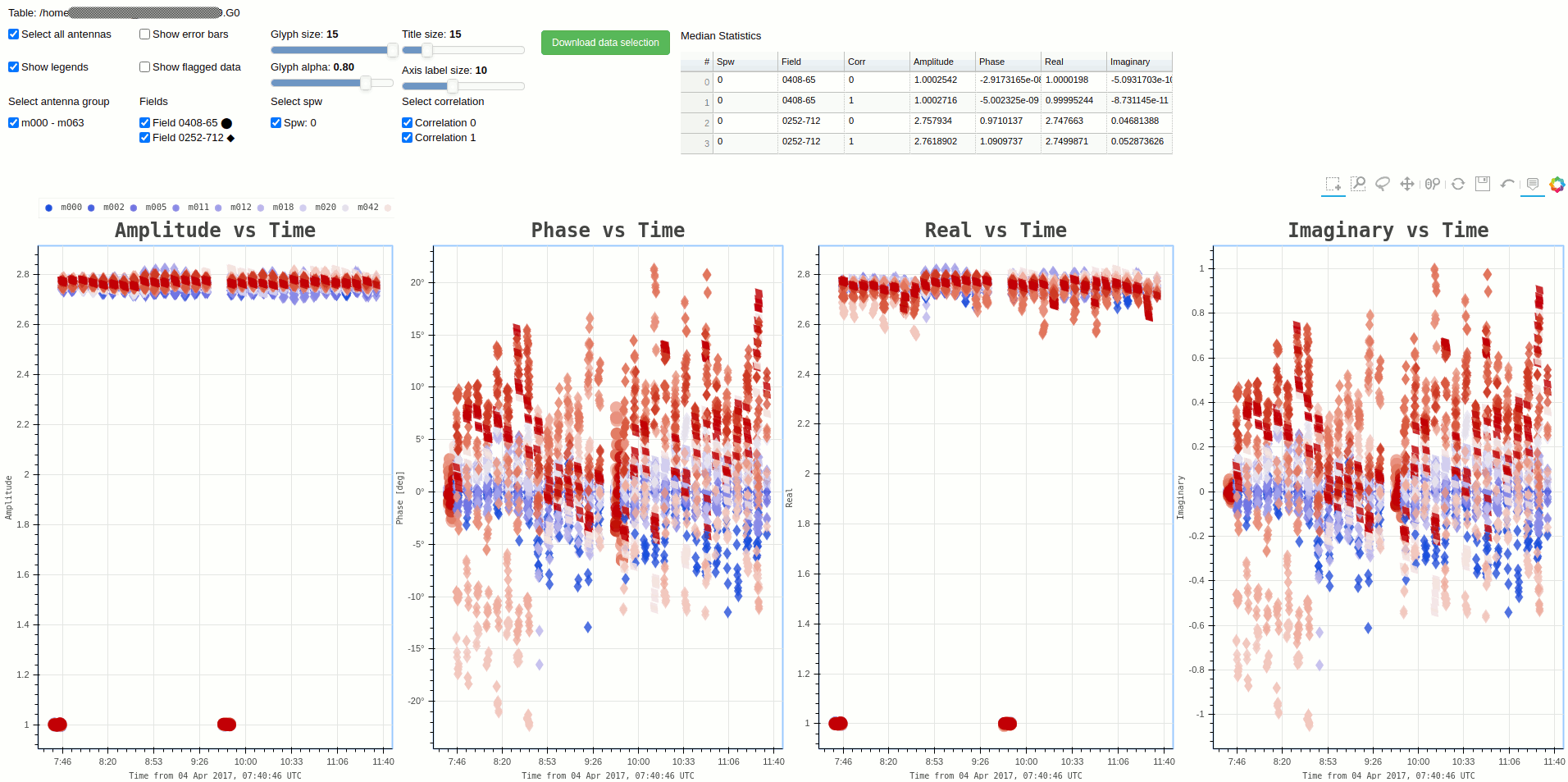
Command: ragavi-gains --table test.B0 --doplot all --htmlname test

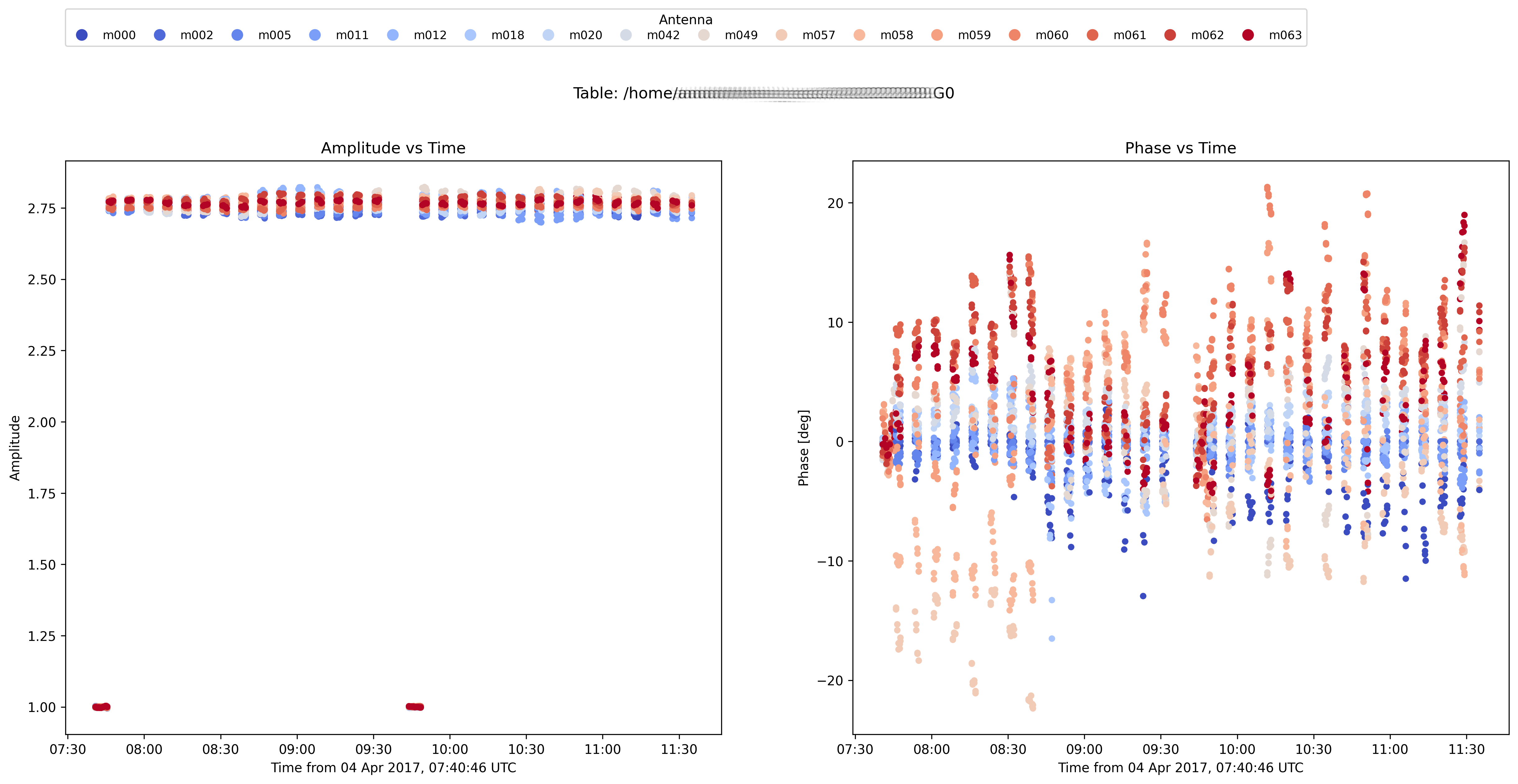
Static plots¶

Command: ragavi-gains --table test.B0 --doplot ap --plotname test.png

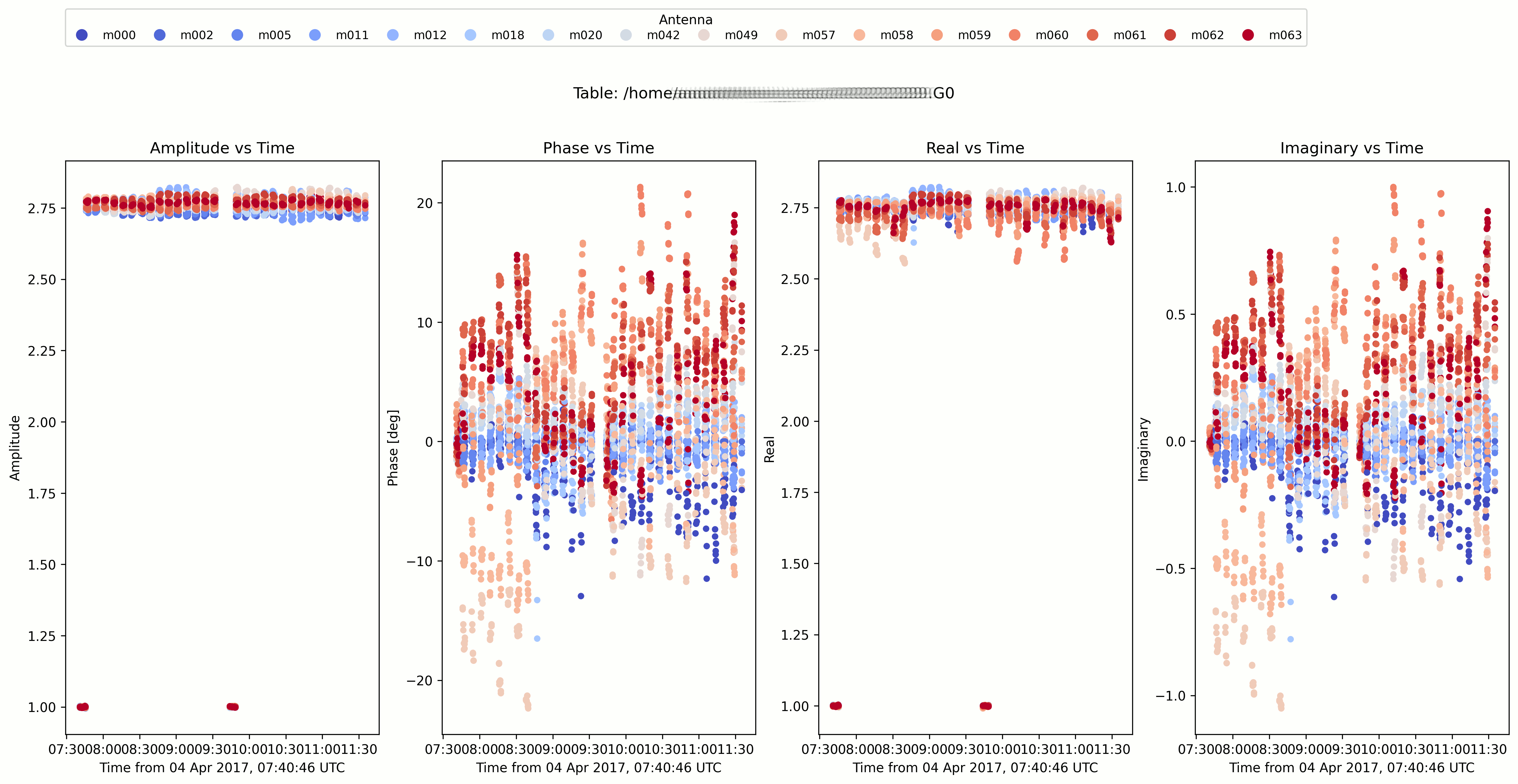
Static plot with ``--doplot ap`` and ``--plotname test.png``

Command: ragavi-gains --table test.B0 --doplot all --plotname test.png

Static plot with ``--doplot all`` and ``--plotname test.png``

Jupyter Notebook function¶

ragavi.ragavi.plot_table(**kwargs)¶

Plot gain tables within Jupyter notebooks. Parameter names correspond to the long names of each argument (i.e those with –) from the ragavi-vis command line help

Parameters:

table (str or list) – The table (list of tables) to be plotted.
ant (str, optional) – Plot only specific antennas, or comma-separated list of antennas.
corr (int, optional) – Correlation index to plot. Can be a single integer or comma separated integers e.g “0,2”. Defaults to all.
cmap (str, optional) – Matplotlib colour map to use for antennas. Default is coolwarm
ddid (int) – SPECTRAL_WINDOW_ID or ddid number. Defaults to all
doplot (str, optional) – Plot complex values as amp and phase (ap) or real and imag (ri). Default is “ap”.
field (str, optional) – Field ID(s) / NAME(s) to plot. Can be specified as “0”, “0,2,4”, “0~3” (inclusive range), “0:3” (exclusive range), “3:” (from 3 to last) or using a field name or comma separated field names. Defaults to all.
k-xaxis (str) – Choose the x-xaxis for the K table. Valid choices are: time or antenna. Defaults to time.
taql (str, optional) – TAQL where clause
t0 (int, optional) – Minimum time [in seconds] to plot. Default is full range
t1 (int, optional) – Maximum time [in seconds] to plot. Default is full range

ragavi-gains¶